This page shows some examples of Jsrtaa being used, along with the Java code to do so. Note that the command line interface can do these as well, though it is obviously not as full-fledged as using the library directly.
First, let's do a simple resize of an image, which happens to be one of my favourite paintings, using bilinear and bicubic interpolation. Here's the original:

				 // Resize by interpolation
				 final ImageTTAA orig = new ImageTTAA(PATH + "5.jpg");
				 ImageTTAA smaller = Interpolation.bilinearInterpolate(orig, orig.width/2, orig.height/2);
				 smaller.saveAs(PATH + "small.png"); // smaller image
				 ImageTTAA interped = Interpolation.bicubicInterpolate(smaller, orig.width, orig.height);
				 interped.saveAs(PATH + "big.png"); // back to full size
Here's the output


What about animated GIFs? Let's resize and Gaussian blur one:


			 GifTTAA gif = new GifTTAA(new File(PATH + "11.gif"));
			 DiscreteKernel g = new NormedGaussianBlurKernel(2,3); // sigma = 2, radius = 3
			 for(int i = 0; i < gif.getNumImages(); ++i){
				 ImageTTAA blurred = SignalProcessing.convolve(gif.getImage(i), g); // blur the frame
				 gif.setImage(i, Interpolation.piecewiseBicubicAkimaSplineInterpolate(blurred, 300, 190)); // resize it
			 }
			 gif.saveAs(PATH + "test_2.gif");
Let's look at noising and denoising. First, the original image:

				// Add noise to an image after resizing it
				ImageTTAA img = Interpolation.piecewiseBicubicAkimaSplineInterpolate(new ImageTTAA(PATH + "1.jpg"),(int)(375*1.5),(int)(300*1.5));
				img.saveAs(PATH + "noiseless2.jpg");
				ImageTTAA noisy = Noise.addGaussianNoiseToImage(img , 0, 20); // mu = 0, sigma = 25
				noisy.saveAs(PATH + "gaussNoise2.jpg");
				// Denoise it with the bilateral filter
				ImageTTAA denoised = BilateralFilter.denoiseByBilateralFilter(noisy, 50, 20, 20); // h, rho, radius
				denoised.saveAs(PATH + "bilatDenoise3.png");
Note the edge preservation in the denoised image!


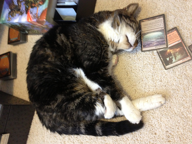
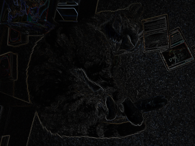
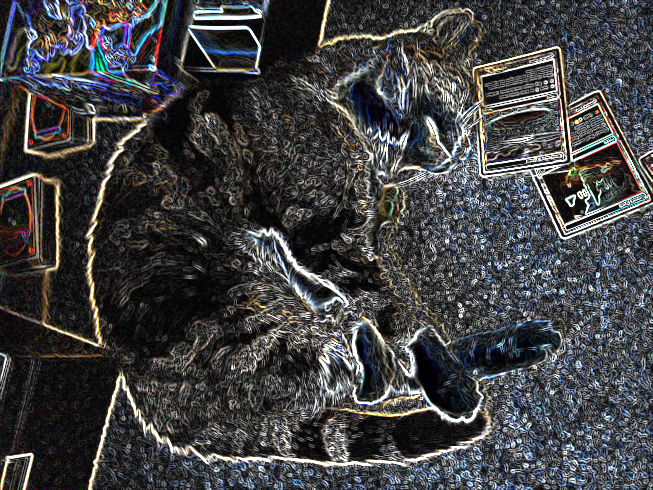
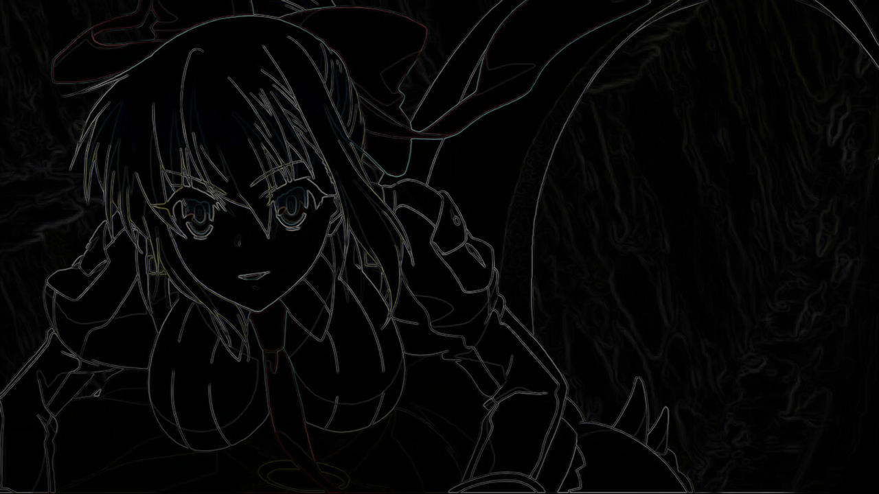
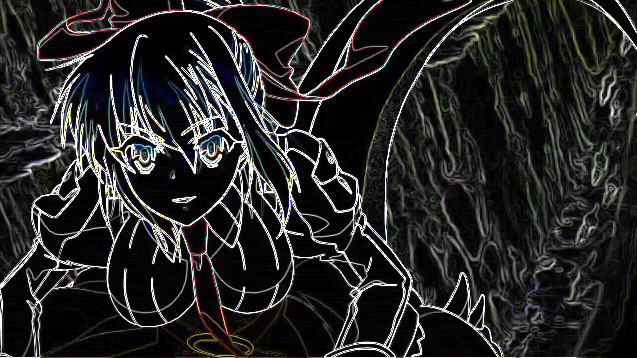
Using this code (for the first image):
				LayeredMatrix m = (new ImageTTAA(PATH + "2.jpg")).convertToLayeredMatrix();
				 // Real-valued representation of an image
				 VectorCalculus.sobelGradientMagnitude(m).convertToImageTTAA().saveAs(PATH + "sobelGrad2.png");
				 VectorCalculus.generateGradientMagnitudeImage(m.convertToImageTTAA()).saveAs(PATH + "defaultGrad2.png");
Now let's look at the Gaussian and mean curvature of the image we denoised above:
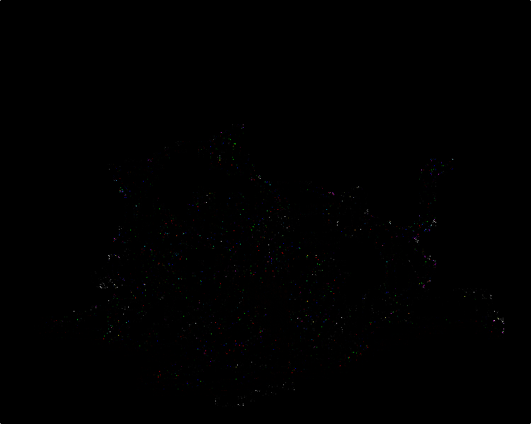
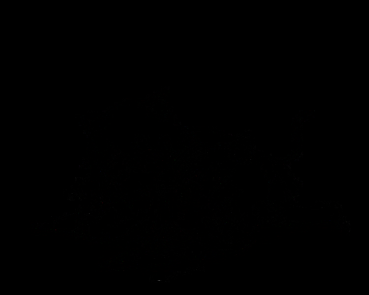
Kind of hard to see anything eh? Let's log normalize it. Now you can at least see the outlines.
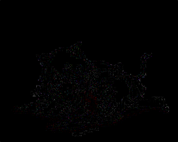
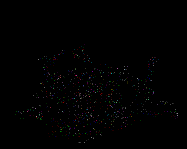
And let's also show the Laplacian over the image:

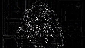
All these transformations are coded as follows:
				 // Curvatures
				 LayeredMatrix c = (new ImageTTAA(PATH + "1.jpg")).convertToLayeredMatrix();
				 ImageTTAA gc = DifferentialGeometry.gaussianCurvature(c).convertToImageTTAA();
				 ImageTTAA mc = DifferentialGeometry.meanCurvature(c).convertToImageTTAA();
				 gc.saveAs(PATH + "gaussCurv.png");
				 mc.saveAs(PATH + "meanCurv.png");
				 // They're pretty faint, so log norm them
				 gc.generateLogNormedImage().saveAs(PATH + "gaussCurv-lognorm.png");
				 mc.generateLogNormedImage().saveAs(PATH + "meanCurv-lognorm.png");
				 // Laplacian
				 LayeredMatrix forLap = (new ImageTTAA(PATH + "4.jpg")).convertToLayeredMatrix();
				 VectorCalculus.laplacianMatrix(forLap).convertToImageTTAA().generateLogNormedImage().saveAs(PATH + "lap2-log.png");
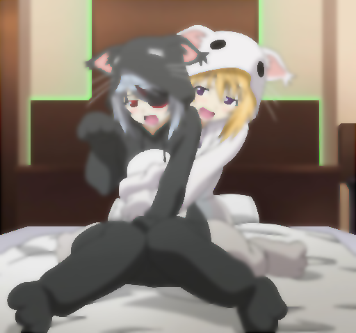
Now, let's look at the anisotropic diffusion methods. Note the preservation of edges as the pixels bleed everywhere as if it were diffusing ink, and how the stronger edges better stop the diffusion. In particular, let's see the Perona-Malik algorithm in action:
			 // Perona-Malik diffusion
			 BufferedImage bi = ImageIO.read(new File(PATH + "3.jpg")); // Convert from a BufferedImage for fun
			 ImageTTAA imgToDiffuse = ImageConvert.convertBufferedImageToImageTtaa(bi);
			 ImageWrite.writeImage( // write it out a different way for fun
				PeronaMalikAnisotropicDiffusion.runPeronaMalikAnisotropicDiffusionOnImage(
					imgToDiffuse, 40, 25, 0.65, PeronaMalikDiffusionConductanceType.EXP, false
				) , // img, k, numIters, lambda, g, smoothBeforeGradient?
				PATH + "diffused4.png" // output file name
			 );

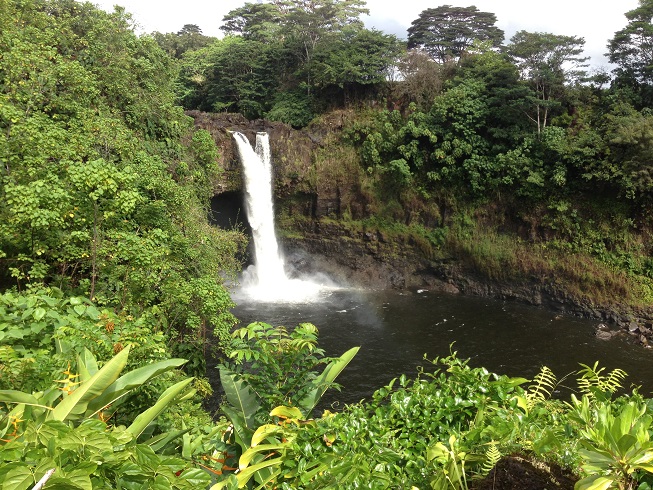
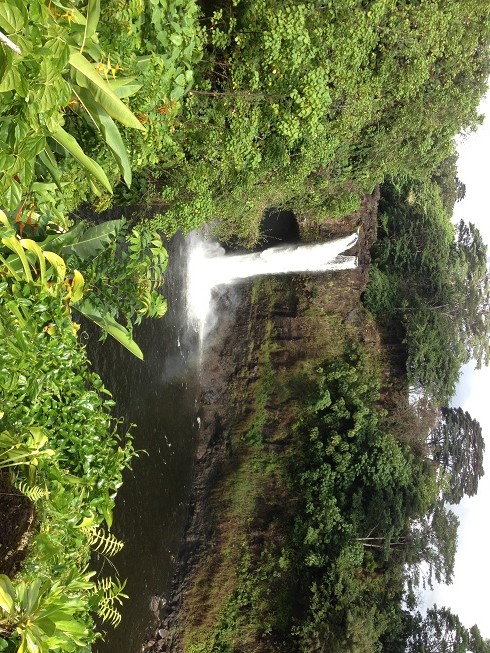
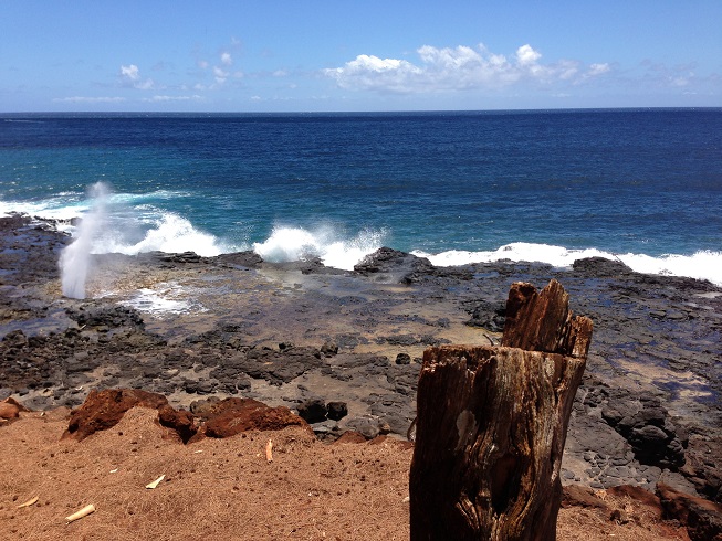
Lastly, let's look at the image distance calculators, using RMSE and Jensen-Shannon divergence. Here's the images:
				 ImageTTAA i1 = Interpolation.bilinearInterpolate(new ImageTTAA(PATH + "6.jpg"),550,550);
				 ImageTTAA i1_rot = Interpolation.bilinearInterpolate(new ImageTTAA(PATH + "6-rot.jpg"),550,550);
				 ImageTTAA i2 = Interpolation.bilinearInterpolate(new ImageTTAA(PATH + "7.jpg"),550,550);
				 i1.saveAs(PATH + "i1.png");
				 i1_rot.saveAs(PATH + "i1_rot.png");
				 i2.saveAs(PATH + "i2.png");
				 System.out.println(ImageMetrics.rmse(i1, i2));
				 System.out.println(ImageMetrics.rmse(i1, i1_rot));
				 System.out.println(ImageMetrics.computeIndependentJensenShannonDivergence(i1, i2));
				 System.out.println(ImageMetrics.computeIndependentJensenShannonDivergence(i1, i1_rot));
This outputs: 11.205015997136218, 10.526272120056143, 0.16143498466910586, 0.013319404644832904. Notice how the rmse thinks that the rotated image is as different from the original as it is from the completely different image, whereas the information-theoretic metric considers the rotated and original images very similar.